01.chipotle Exercises

Ex2 - Getting and Knowing your Data

This time we are going to pull data directly from the internet. Special thanks to: https://github.com/justmarkham for sharing the dataset and materials.

Step 1. Import the necessary libraries

import pandas as pd
import numpy as np

Step 2. Import the dataset from this address.

Step 3. Assign it to a variable called chipo.

chipo = pd.read_csv('https://raw.githubusercontent.com/justmarkham/DAT8/master/data/chipotle.tsv', sep= '\t')

Step 4. See the first 10 entries

chipo.head(10)

	order_id	quantity	item_name	choice_description	item_price
0	1	1	Chips and Fresh Tomato Salsa	NaN	$2.39
1	1	1	Izze	[Clementine]	$3.39
2	1	1	Nantucket Nectar	[Apple]	$3.39
3	1	1	Chips and Tomatillo-Green Chili Salsa	NaN	$2.39
4	2	2	Chicken Bowl	[Tomatillo-Red Chili Salsa (Hot), [Black Beans...	$16.98
5	3	1	Chicken Bowl	[Fresh Tomato Salsa (Mild), [Rice, Cheese, Sou...	$10.98
6	3	1	Side of Chips	NaN	$1.69
7	4	1	Steak Burrito	[Tomatillo Red Chili Salsa, [Fajita Vegetables...	$11.75
8	4	1	Steak Soft Tacos	[Tomatillo Green Chili Salsa, [Pinto Beans, Ch...	$9.25
9	5	1	Steak Burrito	[Fresh Tomato Salsa, [Rice, Black Beans, Pinto...	$9.25

Step 5. What is the number of observations in the dataset?

# Solution 1

chipo.info()

<class 'pandas.core.frame.DataFrame'>
RangeIndex: 4622 entries, 0 to 4621
Data columns (total 5 columns):
 #   Column              Non-Null Count  Dtype 
---  ------              --------------  ----- 
 0   order_id            4622 non-null   int64 
 1   quantity            4622 non-null   int64 
 2   item_name           4622 non-null   object
 3   choice_description  3376 non-null   object
 4   item_price          4622 non-null   object
dtypes: int64(2), object(3)
memory usage: 180.7+ KB

# Solution 2

chipo.shape

(4622, 5)

Step 6. What is the number of columns in the dataset?

chipo.shape[1]

Step 7. Print the name of all the columns.

chipo.head(0)
##chipo.columns

	order_id	quantity	item_name	choice_description	item_price

Step 8. How is the dataset indexed?

chipo.index

RangeIndex(start=0, stop=4622, step=1)

Step 9. Which was the most-ordered item?

chipo.groupby(by="item_name").sum().sort_values('quantity',ascending=False).head(1)

	order_id	quantity	choice_description	item_price
item_name
Chicken Bowl	713926	761	[Tomatillo-Red Chili Salsa (Hot), [Black Beans...	$16.98 $10.98 $11.25 $8.75 $8.49 $11.25 $8.75 ...

Step 10. For the most-ordered item, how many items were ordered?

chipo.groupby(by="item_name").sum().sort_values('quantity',ascending=False).head(1)

	order_id	quantity	choice_description	item_price
item_name
Chicken Bowl	713926	761	[Tomatillo-Red Chili Salsa (Hot), [Black Beans...	$16.98 $10.98 $11.25 $8.75 $8.49 $11.25 $8.75 ...

Step 11. What was the most ordered item in the choice_description column?

chipo.groupby(by="choice_description").sum().sort_values('quantity',ascending=False).head(1)

	order_id	quantity	item_name	item_price
choice_description
[Diet Coke]	123455	159	Canned SodaCanned SodaCanned Soda6 Pack Soft D...	$2.18 $1.09 $1.09 $6.49 $2.18 $1.25 $1.09 $6.4...

Step 12. How many items were orderd in total?

chipo.item_name.count()

Step 13. Turn the item price into a float

Step 13.a. Check the item price type

chipo.item_price.dtype

dtype('O')

Step 13.b. Create a lambda function and change the type of item price

dollarizer = lambda x: float(x[1:-1])
chipo.item_price = chipo.item_price.apply(dollarizer)

Step 13.c. Check the item price type

chipo.item_price.dtype

dtype('float64')

Step 14. How much was the revenue for the period in the dataset?

revenue =  (chipo.item_price * chipo.quantity).sum()
print('Revenue is : $ '+ str(revenue))

Revenue is : $ 39237.02

Step 15. How many orders were made in the period?

chipo.order_id.value_counts().count()

Step 16. What is the average revenue amount per order?

# Solution 1

chipo['revenue'] = chipo['quantity'] * chipo['item_price']
order_grouped = chipo.groupby(by=['order_id']).sum()
order_grouped['revenue'].mean()

21.39423118865867

# Solution 2

chipo.groupby(by=['order_id']).sum()['revenue'].mean()

21.39423118865867

Step 17. How many different items are sold?

chipo.item_name.value_counts().count()

Source: Ex2 - Getting and Knowing your Data

01.occupion Exercises

Ex3 - Getting and Knowing your Data

This time we are going to pull data directly from the internet. Special thanks to: https://github.com/justmarkham for sharing the dataset and materials.

Step 1. Import the necessary libraries

import pandas as pd

Step 2. Import the dataset from this address.

Step 3. Assign it to a variable called users and use the ‘user_id’ as index

users = pd.read_csv('https://raw.githubusercontent.com/justmarkham/DAT8/master/data/u.user', sep='|', index_col='user_id')

Step 4. See the first 25 entries

users.head(25)

	age	gender	occupation	zip_code
user_id
1	24	M	technician	85711
2	53	F	other	94043
3	23	M	writer	32067
4	24	M	technician	43537
5	33	F	other	15213
6	42	M	executive	98101
7	57	M	administrator	91344
8	36	M	administrator	05201
9	29	M	student	01002
10	53	M	lawyer	90703
11	39	F	other	30329
12	28	F	other	06405
13	47	M	educator	29206
14	45	M	scientist	55106
15	49	F	educator	97301
16	21	M	entertainment	10309
17	30	M	programmer	06355
18	35	F	other	37212
19	40	M	librarian	02138
20	42	F	homemaker	95660
21	26	M	writer	30068
22	25	M	writer	40206
23	30	F	artist	48197
24	21	F	artist	94533
25	39	M	engineer	55107

Step 5. See the last 10 entries

users.tail(10)

	age	gender	occupation	zip_code
user_id
934	61	M	engineer	22902
935	42	M	doctor	66221
936	24	M	other	32789
937	48	M	educator	98072
938	38	F	technician	55038
939	26	F	student	33319
940	32	M	administrator	02215
941	20	M	student	97229
942	48	F	librarian	78209
943	22	M	student	77841

Step 6. What is the number of observations in the dataset?

users.shape[0]

Step 7. What is the number of columns in the dataset?

users.shape[1]

Step 8. Print the name of all the columns.

users.columns

Index(['age', 'gender', 'occupation', 'zip_code'], dtype='object')

Step 9. How is the dataset indexed?

# "the index" (aka "the labels")    
# 【索引，又被称为标签】
users.index

Index([  1,   2,   3,   4,   5,   6,   7,   8,   9,  10,
       ...
       934, 935, 936, 937, 938, 939, 940, 941, 942, 943],
      dtype='int64', name='user_id', length=943)

Step 10. What is the data type of each column?

users.dtypes

age            int64
gender        object
occupation    object
zip_code      object
dtype: object

Step 11. Print only the occupation column

users['occupation']

user_id
1         technician
2              other
3             writer
4         technician
5              other
           ...      
939          student
940    administrator
941          student
942        librarian
943          student
Name: occupation, Length: 943, dtype: object

Step 12. How many different occupations are in this dataset?

users.occupation.nunique()
#or by using value_counts() which returns the count of unique elements
#users.occupation.value_counts().count()

Step 13. What is the most frequent occupation?

#Because "most" is asked
users.occupation.value_counts().head(1).index[0]

#or
#to have the top 5

# users.occupation.value_counts().head()

'student'

Step 14. Summarize the DataFrame.

users.describe() #Notice: by default, only the numeric columns are returned.

	age
count	943.000000
mean	34.051962
std	12.192740
min	7.000000
25%	25.000000
50%	31.000000
75%	43.000000
max	73.000000

Step 15. Summarize all the columns

users.describe(include = "all") #Notice: By default, only the numeric columns are returned.

	age	gender	occupation	zip_code
count	943.000000	943	943	943
unique	NaN	2	21	795
top	NaN	M	student	55414
freq	NaN	670	196	9
mean	34.051962	NaN	NaN	NaN
std	12.192740	NaN	NaN	NaN
min	7.000000	NaN	NaN	NaN
25%	25.000000	NaN	NaN	NaN
50%	31.000000	NaN	NaN	NaN
75%	43.000000	NaN	NaN	NaN
max	73.000000	NaN	NaN	NaN

Step 16. Summarize only the occupation column

users.occupation.describe()

count         943
unique         21
top       student
freq          196
Name: occupation, dtype: object

Step 17. What is the mean age of users?

round(users.age.mean())

Step 18. What is the age with least occurrence?

users.age.value_counts().tail() #7, 10, 11, 66 and 73 years -> only 1 occurrence

age
7     1
66    1
11    1
10    1
73    1
Name: count, dtype: int64

Source: Ex3 - Getting and Knowing your Data

01.world food facts Exercises

Exercise 1

Step 1. Go to https://www.kaggle.com/openfoodfacts/world-food-facts/data

Step 2. Download the dataset to your computer and unzip it.

Step 3. Use the tsv file and assign it to a dataframe called food

import pandas as pd
import numpy as np
food = pd.read_csv('en.openfoodfacts.org.products.tsv',sep='\t')

Step 4. See the first 5 entries

food.head()

	code	url	creator	created_t	created_datetime	last_modified_t	last_modified_datetime	product_name	generic_name	quantity	...	fruits-vegetables-nuts_100g	fruits-vegetables-nuts-estimate_100g	collagen-meat-protein-ratio_100g	cocoa_100g	chlorophyl_100g	carbon-footprint_100g	nutrition-score-fr_100g	nutrition-score-uk_100g	glycemic-index_100g	water-hardness_100g
0	3087	http://world-en.openfoodfacts.org/product/0000...	openfoodfacts-contributors	1474103866	2016-09-17T09:17:46Z	1474103893	2016-09-17T09:18:13Z	Farine de blé noir	NaN	1kg	...	NaN	NaN	NaN	NaN	NaN	NaN	NaN	NaN	NaN	NaN
1	4530	http://world-en.openfoodfacts.org/product/0000...	usda-ndb-import	1489069957	2017-03-09T14:32:37Z	1489069957	2017-03-09T14:32:37Z	Banana Chips Sweetened (Whole)	NaN	NaN	...	NaN	NaN	NaN	NaN	NaN	NaN	14.0	14.0	NaN	NaN
2	4559	http://world-en.openfoodfacts.org/product/0000...	usda-ndb-import	1489069957	2017-03-09T14:32:37Z	1489069957	2017-03-09T14:32:37Z	Peanuts	NaN	NaN	...	NaN	NaN	NaN	NaN	NaN	NaN	0.0	0.0	NaN	NaN
3	16087	http://world-en.openfoodfacts.org/product/0000...	usda-ndb-import	1489055731	2017-03-09T10:35:31Z	1489055731	2017-03-09T10:35:31Z	Organic Salted Nut Mix	NaN	NaN	...	NaN	NaN	NaN	NaN	NaN	NaN	12.0	12.0	NaN	NaN
4	16094	http://world-en.openfoodfacts.org/product/0000...	usda-ndb-import	1489055653	2017-03-09T10:34:13Z	1489055653	2017-03-09T10:34:13Z	Organic Polenta	NaN	NaN	...	NaN	NaN	NaN	NaN	NaN	NaN	NaN	NaN	NaN	NaN

5 rows × 163 columns

Step 5. What is the number of observations in the dataset?

food.shape[0]

Step 6. What is the number of columns in the dataset?

food.shape[1]
food.info()

<class 'pandas.core.frame.DataFrame'>
RangeIndex: 356027 entries, 0 to 356026
Columns: 163 entries, code to water-hardness_100g
dtypes: float64(107), object(56)
memory usage: 442.8+ MB

Step 7. Print the name of all the columns.

food.columns

Index(['code', 'url', 'creator', 'created_t', 'created_datetime',
       'last_modified_t', 'last_modified_datetime', 'product_name',
       'generic_name', 'quantity',
       ...
       'fruits-vegetables-nuts_100g', 'fruits-vegetables-nuts-estimate_100g',
       'collagen-meat-protein-ratio_100g', 'cocoa_100g', 'chlorophyl_100g',
       'carbon-footprint_100g', 'nutrition-score-fr_100g',
       'nutrition-score-uk_100g', 'glycemic-index_100g',
       'water-hardness_100g'],
      dtype='object', length=163)

Step 8. What is the name of 105th column?

food.columns[104]

'-glucose_100g'

Step 9. What is the type of the observations of the 105th column?

food.dtypes[food.columns[104]]

dtype('float64')

Step 10. How is the dataset indexed?

food.index

RangeIndex(start=0, stop=356027, step=1)

Step 11. What is the product name of the 19th observation?

food.values[18][7]

'Lotus Organic Brown Jasmine Rice'

Source: Exercise 1

02_chipotle_Exercises

Ex1 - Filtering and Sorting Data

This time we are going to pull data directly from the internet. Special thanks to: https://github.com/justmarkham for sharing the dataset and materials.

Step 1. Import the necessary libraries

import pandas as pd
import numpy as np

Step 2. Import the dataset from this address.

Step 3. Assign it to a variable called chipo.

chipo = pd.read_csv('https://raw.githubusercontent.com/justmarkham/DAT8/master/data/chipotle.tsv',sep='\t')
chipo.head()

	order_id	quantity	item_name	choice_description	item_price
0	1	1	Chips and Fresh Tomato Salsa	NaN	$2.39
1	1	1	Izze	[Clementine]	$3.39
2	1	1	Nantucket Nectar	[Apple]	$3.39
3	1	1	Chips and Tomatillo-Green Chili Salsa	NaN	$2.39
4	2	2	Chicken Bowl	[Tomatillo-Red Chili Salsa (Hot), [Black Beans...	$16.98

Step 4. How many products cost more than $10.00?

chipo['item_price'] = chipo['item_price'].apply(lambda x:float(x[1:]))

chipo_4 = chipo.drop_duplicates(['item_name','quantity'])

chipo_4 = chipo_4[chipo_4.quantity == 1]

chipo_4[chipo_4.item_price > 10].item_name.nunique()

Step 5. What is the price of each item?

print a data frame with only two columns item_name and item_price

chipo_5 = chipo.drop_duplicates(['item_name'])
chipo_5 = chipo_5[chipo_5.quantity == 1]
chipo_5[['item_name','item_price']]

	item_name	item_price
0	Chips and Fresh Tomato Salsa	2.39
1	Izze	3.39
2	Nantucket Nectar	3.39
3	Chips and Tomatillo-Green Chili Salsa	2.39
6	Side of Chips	1.69
7	Steak Burrito	11.75
8	Steak Soft Tacos	9.25
10	Chips and Guacamole	4.45
11	Chicken Crispy Tacos	8.75
12	Chicken Soft Tacos	8.75
16	Chicken Burrito	8.49
21	Barbacoa Burrito	8.99
27	Carnitas Burrito	8.99
33	Carnitas Bowl	8.99
34	Bottled Water	1.09
38	Chips and Tomatillo Green Chili Salsa	2.95
39	Barbacoa Bowl	11.75
40	Chips	2.15
44	Chicken Salad Bowl	8.75
54	Steak Bowl	8.99
56	Barbacoa Soft Tacos	9.25
57	Veggie Burrito	11.25
62	Veggie Bowl	11.25
92	Steak Crispy Tacos	9.25
111	Chips and Tomatillo Red Chili Salsa	2.95
168	Barbacoa Crispy Tacos	11.75
186	Veggie Salad Bowl	11.25
191	Chips and Roasted Chili-Corn Salsa	2.39
233	Chips and Roasted Chili Corn Salsa	2.95
237	Carnitas Soft Tacos	9.25
250	Chicken Salad	10.98
263	Canned Soft Drink	1.25
298	6 Pack Soft Drink	6.49
300	Chips and Tomatillo-Red Chili Salsa	2.39
510	Burrito	7.40
520	Crispy Tacos	7.40
554	Carnitas Crispy Tacos	9.25
664	Steak Salad	8.99
674	Chips and Mild Fresh Tomato Salsa	3.00
738	Veggie Soft Tacos	11.25
1132	Carnitas Salad Bowl	11.89
1229	Barbacoa Salad Bowl	11.89
1414	Salad	7.40
1653	Veggie Crispy Tacos	8.49
1694	Veggie Salad	8.49
3750	Carnitas Salad	8.99

Step 6. Sort by the name of the item

chipo_5[['item_name','item_price']].sort_values(by='item_name')

	item_name	item_price
298	6 Pack Soft Drink	6.49
39	Barbacoa Bowl	11.75
21	Barbacoa Burrito	8.99
168	Barbacoa Crispy Tacos	11.75
1229	Barbacoa Salad Bowl	11.89
56	Barbacoa Soft Tacos	9.25
34	Bottled Water	1.09
510	Burrito	7.40
263	Canned Soft Drink	1.25
33	Carnitas Bowl	8.99
27	Carnitas Burrito	8.99
554	Carnitas Crispy Tacos	9.25
3750	Carnitas Salad	8.99
1132	Carnitas Salad Bowl	11.89
237	Carnitas Soft Tacos	9.25
16	Chicken Burrito	8.49
11	Chicken Crispy Tacos	8.75
250	Chicken Salad	10.98
44	Chicken Salad Bowl	8.75
12	Chicken Soft Tacos	8.75
40	Chips	2.15
0	Chips and Fresh Tomato Salsa	2.39
10	Chips and Guacamole	4.45
674	Chips and Mild Fresh Tomato Salsa	3.00
233	Chips and Roasted Chili Corn Salsa	2.95
191	Chips and Roasted Chili-Corn Salsa	2.39
38	Chips and Tomatillo Green Chili Salsa	2.95
111	Chips and Tomatillo Red Chili Salsa	2.95
3	Chips and Tomatillo-Green Chili Salsa	2.39
300	Chips and Tomatillo-Red Chili Salsa	2.39
520	Crispy Tacos	7.40
1	Izze	3.39
2	Nantucket Nectar	3.39
1414	Salad	7.40
6	Side of Chips	1.69
54	Steak Bowl	8.99
7	Steak Burrito	11.75
92	Steak Crispy Tacos	9.25
664	Steak Salad	8.99
8	Steak Soft Tacos	9.25
62	Veggie Bowl	11.25
57	Veggie Burrito	11.25
1653	Veggie Crispy Tacos	8.49
1694	Veggie Salad	8.49
186	Veggie Salad Bowl	11.25
738	Veggie Soft Tacos	11.25

Step 7. What was the quantity of the most expensive item ordered?

chipo_5.sort_values(by='item_name').tail(1)

	order_id	quantity	item_name	choice_description	item_price
738	304	1	Veggie Soft Tacos	[Tomatillo Red Chili Salsa, [Fajita Vegetables...	11.25

Step 8. How many times was a Veggie Salad Bowl ordered?

len(chipo[chipo.item_name == 'Veggie Salad Bowl'])

Step 9. How many times did someone order more than one Canned Soda?

len(chipo[(chipo.item_name == 'Canned Soda') & (chipo.quantity > 1)])

Source: Ex1 - Filtering and Sorting Data

02_euro12_Exercises

Ex2 - Filtering and Sorting Data

This time we are going to pull data directly from the internet.

Step 1. Import the necessary libraries

import pandas as pd

Step 2. Import the dataset from this address.

Step 3. Assign it to a variable called euro12.

euro12 = pd.read_csv('https://raw.githubusercontent.com/guipsamora/pandas_exercises/master/02_Filtering_%26_Sorting/Euro12/Euro_2012_stats_TEAM.csv', sep=',')
euro12

	Team	Goals	Shots on target	Shots off target	Shooting Accuracy	% Goals-to-shots	Total shots (inc. Blocked)	Hit Woodwork	Penalty goals	Penalties not scored	...	Saves made	Saves-to-shots ratio	Fouls Won	Fouls Conceded	Offsides	Yellow Cards	Red Cards	Subs on	Subs off	Players Used
0	Croatia	4	13	12	51.9%	16.0%	32	0	0	0	...	13	81.3%	41	62	2	9	0	9	9	16
1	Czech Republic	4	13	18	41.9%	12.9%	39	0	0	0	...	9	60.1%	53	73	8	7	0	11	11	19
2	Denmark	4	10	10	50.0%	20.0%	27	1	0	0	...	10	66.7%	25	38	8	4	0	7	7	15
3	England	5	11	18	50.0%	17.2%	40	0	0	0	...	22	88.1%	43	45	6	5	0	11	11	16
4	France	3	22	24	37.9%	6.5%	65	1	0	0	...	6	54.6%	36	51	5	6	0	11	11	19
5	Germany	10	32	32	47.8%	15.6%	80	2	1	0	...	10	62.6%	63	49	12	4	0	15	15	17
6	Greece	5	8	18	30.7%	19.2%	32	1	1	1	...	13	65.1%	67	48	12	9	1	12	12	20
7	Italy	6	34	45	43.0%	7.5%	110	2	0	0	...	20	74.1%	101	89	16	16	0	18	18	19
8	Netherlands	2	12	36	25.0%	4.1%	60	2	0	0	...	12	70.6%	35	30	3	5	0	7	7	15
9	Poland	2	15	23	39.4%	5.2%	48	0	0	0	...	6	66.7%	48	56	3	7	1	7	7	17
10	Portugal	6	22	42	34.3%	9.3%	82	6	0	0	...	10	71.5%	73	90	10	12	0	14	14	16
11	Republic of Ireland	1	7	12	36.8%	5.2%	28	0	0	0	...	17	65.4%	43	51	11	6	1	10	10	17
12	Russia	5	9	31	22.5%	12.5%	59	2	0	0	...	10	77.0%	34	43	4	6	0	7	7	16
13	Spain	12	42	33	55.9%	16.0%	100	0	1	0	...	15	93.8%	102	83	19	11	0	17	17	18
14	Sweden	5	17	19	47.2%	13.8%	39	3	0	0	...	8	61.6%	35	51	7	7	0	9	9	18
15	Ukraine	2	7	26	21.2%	6.0%	38	0	0	0	...	13	76.5%	48	31	4	5	0	9	9	18

16 rows × 35 columns

Step 4. Select only the Goal column.

euro12.Goals

0      4
1      4
2      4
3      5
4      3
5     10
6      5
7      6
8      2
9      2
10     6
11     1
12     5
13    12
14     5
15     2
Name: Goals, dtype: int64

Step 5. How many team participated in the Euro2012?

euro12.shape[0]

Step 6. What is the number of columns in the dataset?

euro12.info()

<class 'pandas.core.frame.DataFrame'>
RangeIndex: 16 entries, 0 to 15
Data columns (total 35 columns):
 #   Column                      Non-Null Count  Dtype  
---  ------                      --------------  -----  
 0   Team                        16 non-null     object 
 1   Goals                       16 non-null     int64  
 2   Shots on target             16 non-null     int64  
 3   Shots off target            16 non-null     int64  
 4   Shooting Accuracy           16 non-null     object 
 5   % Goals-to-shots            16 non-null     object 
 6   Total shots (inc. Blocked)  16 non-null     int64  
 7   Hit Woodwork                16 non-null     int64  
 8   Penalty goals               16 non-null     int64  
 9   Penalties not scored        16 non-null     int64  
 10  Headed goals                16 non-null     int64  
 11  Passes                      16 non-null     int64  
 12  Passes completed            16 non-null     int64  
 13  Passing Accuracy            16 non-null     object 
 14  Touches                     16 non-null     int64  
 15  Crosses                     16 non-null     int64  
 16  Dribbles                    16 non-null     int64  
 17  Corners Taken               16 non-null     int64  
 18  Tackles                     16 non-null     int64  
 19  Clearances                  16 non-null     int64  
 20  Interceptions               16 non-null     int64  
 21  Clearances off line         15 non-null     float64
 22  Clean Sheets                16 non-null     int64  
 23  Blocks                      16 non-null     int64  
 24  Goals conceded              16 non-null     int64  
 25  Saves made                  16 non-null     int64  
 26  Saves-to-shots ratio        16 non-null     object 
 27  Fouls Won                   16 non-null     int64  
 28  Fouls Conceded              16 non-null     int64  
 29  Offsides                    16 non-null     int64  
 30  Yellow Cards                16 non-null     int64  
 31  Red Cards                   16 non-null     int64  
 32  Subs on                     16 non-null     int64  
 33  Subs off                    16 non-null     int64  
 34  Players Used                16 non-null     int64  
dtypes: float64(1), int64(29), object(5)
memory usage: 4.5+ KB

Step 7. View only the columns Team, Yellow Cards and Red Cards and assign them to a dataframe called discipline

discipline = euro12[['Team', 'Yellow Cards', 'Red Cards']]
discipline

	Team	Yellow Cards	Red Cards
0	Croatia	9	0
1	Czech Republic	7	0
2	Denmark	4	0
3	England	5	0
4	France	6	0
5	Germany	4	0
6	Greece	9	1
7	Italy	16	0
8	Netherlands	5	0
9	Poland	7	1
10	Portugal	12	0
11	Republic of Ireland	6	1
12	Russia	6	0
13	Spain	11	0
14	Sweden	7	0
15	Ukraine	5	0

Step 8. Sort the teams by Red Cards, then to Yellow Cards

# 默认是升序排序，设置ascending = False后变为降序排序。
discipline.sort_values(['Red Cards', 'Yellow Cards'], ascending = False)

	Team	Yellow Cards	Red Cards
6	Greece	9	1
9	Poland	7	1
11	Republic of Ireland	6	1
7	Italy	16	0
10	Portugal	12	0
13	Spain	11	0
0	Croatia	9	0
1	Czech Republic	7	0
14	Sweden	7	0
4	France	6	0
12	Russia	6	0
3	England	5	0
8	Netherlands	5	0
15	Ukraine	5	0
2	Denmark	4	0
5	Germany	4	0

Step 9. Calculate the mean Yellow Cards given per Team

round(discipline['Yellow Cards'].mean())

Step 10. Filter teams that scored more than 6 goals

euro12[euro12.Goals > 6]

	Team	Goals	Shots on target	Shots off target	Shooting Accuracy	% Goals-to-shots	Total shots (inc. Blocked)	Hit Woodwork	Penalty goals	Penalties not scored	...	Saves made	Saves-to-shots ratio	Fouls Won	Fouls Conceded	Offsides	Yellow Cards	Red Cards	Subs on	Subs off	Players Used
5	Germany	10	32	32	47.8%	15.6%	80	2	1	0	...	10	62.6%	63	49	12	4	0	15	15	17
13	Spain	12	42	33	55.9%	16.0%	100	0	1	0	...	15	93.8%	102	83	19	11	0	17	17	18

2 rows × 35 columns

Step 11. Select the teams that start with G

euro12[euro12.Team.str.startswith('G')]

	Team	Goals	Shots on target	Shots off target	Shooting Accuracy	% Goals-to-shots	Total shots (inc. Blocked)	Hit Woodwork	Penalty goals	Penalties not scored	...	Saves made	Saves-to-shots ratio	Fouls Won	Fouls Conceded	Offsides	Yellow Cards	Red Cards	Subs on	Subs off	Players Used
5	Germany	10	32	32	47.8%	15.6%	80	2	1	0	...	10	62.6%	63	49	12	4	0	15	15	17
6	Greece	5	8	18	30.7%	19.2%	32	1	1	1	...	13	65.1%	67	48	12	9	1	12	12	20

2 rows × 35 columns

Step 12. Select the first 7 columns

euro12.iloc[: , 0:7]

	Team	Goals	Shots on target	Shots off target	Shooting Accuracy	% Goals-to-shots	Total shots (inc. Blocked)
0	Croatia	4	13	12	51.9%	16.0%	32
1	Czech Republic	4	13	18	41.9%	12.9%	39
2	Denmark	4	10	10	50.0%	20.0%	27
3	England	5	11	18	50.0%	17.2%	40
4	France	3	22	24	37.9%	6.5%	65
5	Germany	10	32	32	47.8%	15.6%	80
6	Greece	5	8	18	30.7%	19.2%	32
7	Italy	6	34	45	43.0%	7.5%	110
8	Netherlands	2	12	36	25.0%	4.1%	60
9	Poland	2	15	23	39.4%	5.2%	48
10	Portugal	6	22	42	34.3%	9.3%	82
11	Republic of Ireland	1	7	12	36.8%	5.2%	28
12	Russia	5	9	31	22.5%	12.5%	59
13	Spain	12	42	33	55.9%	16.0%	100
14	Sweden	5	17	19	47.2%	13.8%	39
15	Ukraine	2	7	26	21.2%	6.0%	38

Step 13. Select all columns except the last 3.

euro12.iloc[: , :-3]

	Team	Goals	Shots on target	Shots off target	Shooting Accuracy	% Goals-to-shots	Total shots (inc. Blocked)	Hit Woodwork	Penalty goals	Penalties not scored	...	Clean Sheets	Blocks	Goals conceded	Saves made	Saves-to-shots ratio	Fouls Won	Fouls Conceded	Offsides	Yellow Cards	Red Cards
0	Croatia	4	13	12	51.9%	16.0%	32	0	0	0	...	0	10	3	13	81.3%	41	62	2	9	0
1	Czech Republic	4	13	18	41.9%	12.9%	39	0	0	0	...	1	10	6	9	60.1%	53	73	8	7	0
2	Denmark	4	10	10	50.0%	20.0%	27	1	0	0	...	1	10	5	10	66.7%	25	38	8	4	0
3	England	5	11	18	50.0%	17.2%	40	0	0	0	...	2	29	3	22	88.1%	43	45	6	5	0
4	France	3	22	24	37.9%	6.5%	65	1	0	0	...	1	7	5	6	54.6%	36	51	5	6	0
5	Germany	10	32	32	47.8%	15.6%	80	2	1	0	...	1	11	6	10	62.6%	63	49	12	4	0
6	Greece	5	8	18	30.7%	19.2%	32	1	1	1	...	1	23	7	13	65.1%	67	48	12	9	1
7	Italy	6	34	45	43.0%	7.5%	110	2	0	0	...	2	18	7	20	74.1%	101	89	16	16	0
8	Netherlands	2	12	36	25.0%	4.1%	60	2	0	0	...	0	9	5	12	70.6%	35	30	3	5	0
9	Poland	2	15	23	39.4%	5.2%	48	0	0	0	...	0	8	3	6	66.7%	48	56	3	7	1
10	Portugal	6	22	42	34.3%	9.3%	82	6	0	0	...	2	11	4	10	71.5%	73	90	10	12	0
11	Republic of Ireland	1	7	12	36.8%	5.2%	28	0	0	0	...	0	23	9	17	65.4%	43	51	11	6	1
12	Russia	5	9	31	22.5%	12.5%	59	2	0	0	...	0	8	3	10	77.0%	34	43	4	6	0
13	Spain	12	42	33	55.9%	16.0%	100	0	1	0	...	5	8	1	15	93.8%	102	83	19	11	0
14	Sweden	5	17	19	47.2%	13.8%	39	3	0	0	...	1	12	5	8	61.6%	35	51	7	7	0
15	Ukraine	2	7	26	21.2%	6.0%	38	0	0	0	...	0	4	4	13	76.5%	48	31	4	5	0

16 rows × 32 columns

Step 14. Present only the Shooting Accuracy from England, Italy and Russia

euro12.loc[euro12.Team.isin(['England', 'Italy', 'Russia']), ['Team','Shooting Accuracy']]

	Team	Shooting Accuracy
3	England	50.0%
7	Italy	43.0%
12	Russia	22.5%

Source: Ex2 - Filtering and Sorting Data

03_chipotle_Exercises

Visualizing Chipotle’s Data

This time we are going to pull data directly from the internet. Special thanks to: https://github.com/justmarkham for sharing the dataset and materials.

Step 1. Import the necessary libraries

import pandas as pd
import matplotlib.pyplot as plt
from collections import Counter

# set this so the graphs open internally
%matplotlib inline

Step 2. Import the dataset from this address.

Step 3. Assign it to a variable called chipo.

chipo = pd.read_csv('https://raw.githubusercontent.com/justmarkham/DAT8/master/data/chipotle.tsv',sep='\t')
chipo

	order_id	quantity	item_name	choice_description	item_price
0	1	1	Chips and Fresh Tomato Salsa	NaN	$2.39
1	1	1	Izze	[Clementine]	$3.39
2	1	1	Nantucket Nectar	[Apple]	$3.39
3	1	1	Chips and Tomatillo-Green Chili Salsa	NaN	$2.39
4	2	2	Chicken Bowl	[Tomatillo-Red Chili Salsa (Hot), [Black Beans...	$16.98
...	...	...	...	...	...
4617	1833	1	Steak Burrito	[Fresh Tomato Salsa, [Rice, Black Beans, Sour ...	$11.75
4618	1833	1	Steak Burrito	[Fresh Tomato Salsa, [Rice, Sour Cream, Cheese...	$11.75
4619	1834	1	Chicken Salad Bowl	[Fresh Tomato Salsa, [Fajita Vegetables, Pinto...	$11.25
4620	1834	1	Chicken Salad Bowl	[Fresh Tomato Salsa, [Fajita Vegetables, Lettu...	$8.75
4621	1834	1	Chicken Salad Bowl	[Fresh Tomato Salsa, [Fajita Vegetables, Pinto...	$8.75

4622 rows × 5 columns

Step 4. See the first 10 entries

chipo.head(10)

	order_id	quantity	item_name	choice_description	item_price
0	1	1	Chips and Fresh Tomato Salsa	NaN	$2.39
1	1	1	Izze	[Clementine]	$3.39
2	1	1	Nantucket Nectar	[Apple]	$3.39
3	1	1	Chips and Tomatillo-Green Chili Salsa	NaN	$2.39
4	2	2	Chicken Bowl	[Tomatillo-Red Chili Salsa (Hot), [Black Beans...	$16.98
5	3	1	Chicken Bowl	[Fresh Tomato Salsa (Mild), [Rice, Cheese, Sou...	$10.98
6	3	1	Side of Chips	NaN	$1.69
7	4	1	Steak Burrito	[Tomatillo Red Chili Salsa, [Fajita Vegetables...	$11.75
8	4	1	Steak Soft Tacos	[Tomatillo Green Chili Salsa, [Pinto Beans, Ch...	$9.25
9	5	1	Steak Burrito	[Fresh Tomato Salsa, [Rice, Black Beans, Pinto...	$9.25

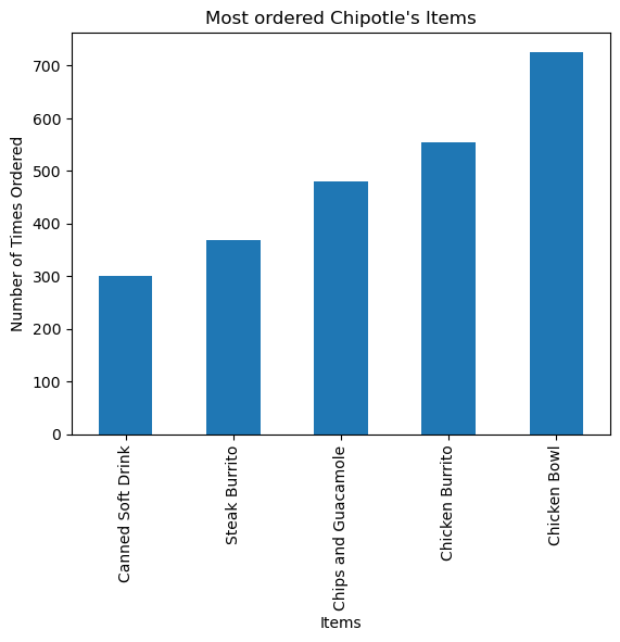
Step 5. Create a histogram of the top 5 items bought

x = chipo.item_name
letter_counts = Counter(x)
df = pd.DataFrame.from_dict(letter_counts, orient='index')
df = df[0].sort_values(ascending = True)[45:50]
df.plot(kind='bar')
plt.xlabel('Items')
plt.ylabel('Number of Times Ordered')
plt.title('Most ordered Chipotle\'s Items')
plt.show()

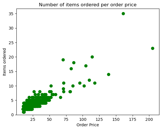
Step 6. Create a scatterplot with the number of items orderered per order price

Hint: Price should be in the X-axis and Items ordered in the Y-axis

chipo.item_price = [float(value[1:-1]) for value in chipo.item_price]

orders = chipo.groupby('order_id').sum()

plt.scatter(x = orders.item_price, y = orders.quantity, s = 50, c = 'green')

plt.xlabel('Order Price')
plt.ylabel('Items ordered')
plt.title('Number of items ordered per order price')
plt.ylim(0)

Step 7. BONUS: Create a question and a graph to answer your own question.

Source: Visualizing Chipotle's Data

03_scores_Exercises

Scores

Introduction:

This time you will create the data.

Exercise based on Chris Albon work, the credits belong to him.

Step 1. Import the necessary libraries

import pandas as pd
import matplotlib.pyplot as plt
import numpy as np

%matplotlib inline

Step 2. Create the DataFrame that should look like the one below.

raw_data = {'first_name': ['Jason', 'Molly', 'Tina', 'Jake', 'Amy'], 
            'last_name': ['Miller', 'Jacobson', 'Ali', 'Milner', 'Cooze'], 
            'female': [0, 1, 1, 0, 1],
            'age': [42, 52, 36, 24, 73], 
            'preTestScore': [4, 24, 31, 2, 3],
            'postTestScore': [25, 94, 57, 62, 70]}

df = pd.DataFrame(raw_data)
df

	first_name	last_name	female	age	preTestScore	postTestScore
0	Jason	Miller	0	42	4	25
1	Molly	Jacobson	1	52	24	94
2	Tina	Ali	1	36	31	57
3	Jake	Milner	0	24	2	62
4	Amy	Cooze	1	73	3	70

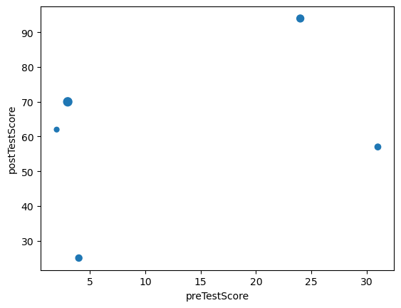
Step 3. Create a Scatterplot of preTestScore and postTestScore, with the size of each point determined by age

Hint: Don’t forget to place the labels

df.plot.scatter(x='preTestScore' , y='postTestScore'  , s=df['age'].values)

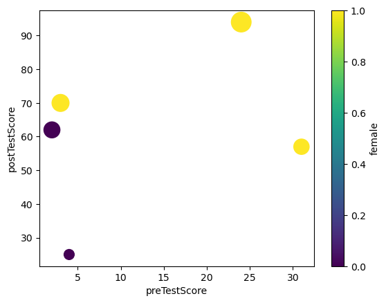
Step 4. Create a Scatterplot of preTestScore and postTestScore.

This time the size should be 4.5 times the postTestScore and the color determined by sex

df.plot.scatter(x='preTestScore' , y='postTestScore' , s=df['postTestScore']*4.5 , c='female' , colormap='viridis')

BONUS: Create your own question and answer it.

Source: Scores

Notebooks

01.chipotle Exercises

Ex2 - Getting and Knowing your Data

Step 1. Import the necessary libraries

Step 2. Import the dataset from this address.

Step 3. Assign it to a variable called chipo.

Step 4. See the first 10 entries

Step 5. What is the number of observations in the dataset?

Step 6. What is the number of columns in the dataset?

Step 7. Print the name of all the columns.

Step 8. How is the dataset indexed?

Step 9. Which was the most-ordered item?

Step 10. For the most-ordered item, how many items were ordered?

Step 11. What was the most ordered item in the choice_description column?

Step 12. How many items were orderd in total?

Step 13. Turn the item price into a float

Step 13.a. Check the item price type

Step 13.b. Create a lambda function and change the type of item price

Step 13.c. Check the item price type

Step 14. How much was the revenue for the period in the dataset?

Step 15. How many orders were made in the period?

Step 16. What is the average revenue amount per order?

Step 17. How many different items are sold?

01.occupion Exercises

Ex3 - Getting and Knowing your Data

Step 1. Import the necessary libraries

Step 2. Import the dataset from this address.

Step 3. Assign it to a variable called users and use the ‘user_id’ as index

Step 4. See the first 25 entries

Step 5. See the last 10 entries

Step 6. What is the number of observations in the dataset?

Step 7. What is the number of columns in the dataset?

Step 8. Print the name of all the columns.

Step 9. How is the dataset indexed?

Step 10. What is the data type of each column?

Step 11. Print only the occupation column

Step 12. How many different occupations are in this dataset?

Step 13. What is the most frequent occupation?

Step 14. Summarize the DataFrame.

Step 15. Summarize all the columns

Step 16. Summarize only the occupation column

Step 17. What is the mean age of users?

Step 18. What is the age with least occurrence?

01.world food facts Exercises

Exercise 1

Step 1. Go to https://www.kaggle.com/openfoodfacts/world-food-facts/data

Step 2. Download the dataset to your computer and unzip it.

Step 3. Use the tsv file and assign it to a dataframe called food

Step 4. See the first 5 entries

Step 5. What is the number of observations in the dataset?

Step 6. What is the number of columns in the dataset?

Step 7. Print the name of all the columns.

Step 8. What is the name of 105th column?

Step 9. What is the type of the observations of the 105th column?

Step 10. How is the dataset indexed?

Step 11. What is the product name of the 19th observation?

02_chipotle_Exercises

Ex1 - Filtering and Sorting Data

Step 1. Import the necessary libraries

Step 2. Import the dataset from this address.

Step 3. Assign it to a variable called chipo.

Step 4. How many products cost more than $10.00?

Step 5. What is the price of each item?

print a data frame with only two columns item_name and item_price

Step 6. Sort by the name of the item

Step 7. What was the quantity of the most expensive item ordered?

Step 8. How many times was a Veggie Salad Bowl ordered?

Step 9. How many times did someone order more than one Canned Soda?

02_euro12_Exercises

Ex2 - Filtering and Sorting Data

Step 1. Import the necessary libraries

Step 2. Import the dataset from this address.

Step 3. Assign it to a variable called euro12.

Step 4. Select only the Goal column.

Step 5. How many team participated in the Euro2012?

Step 6. What is the number of columns in the dataset?

Step 7. View only the columns Team, Yellow Cards and Red Cards and assign them to a dataframe called discipline

Step 8. Sort the teams by Red Cards, then to Yellow Cards

Step 9. Calculate the mean Yellow Cards given per Team

Step 10. Filter teams that scored more than 6 goals